This document is here to give students who are unfamiliar with R or who haven’t used R for a long time some basic familiarity with the language. We will cover the basics of
What is R and why are we using it?
R is a programming language (a syntax for humans to tell computers what to do) and a runtime environment (a program that translates a language into something a computer understands). This puts it in the same family as computer-sciency languages like Python, C++, Java, etc. But what makes R distinct is that it is a programming language designed specifically for statistical analysis, data manipulation, and the creation of figures and charts—i.e. designed specifically for doing science. R (along with its predecessors S and S-plus) has been used by statisticians, mathematicians, and computer scientists since the 1970s, and since about the mid 00s it has gained a considerable following in the social sciences. I am teaching this course using R for a few reasons:
igraph that we will be relying on heavily in this class.Installing R There are many ways to run, and interact with R, but one of the simplest is to use the RStudio interface. RStudio is a bare-bones graphical interface to R that makes a few of the more arcane and common tasks much easier. It also provides a single graphical window where you can write scripts, execute commands, explore your data, see visualsizations, and access documentation.
R and RStudio are installed separately. If you are using an Apple Mac or a Microsoft Windows computer:
Once both of these have run, you should be able to open RStudio.
Note: the remainder of this lab is adapted from Data Carpentry’s “Introduction to R and RStudio” (CC-BY 4.0 by The Carpentries.)
Basic layout
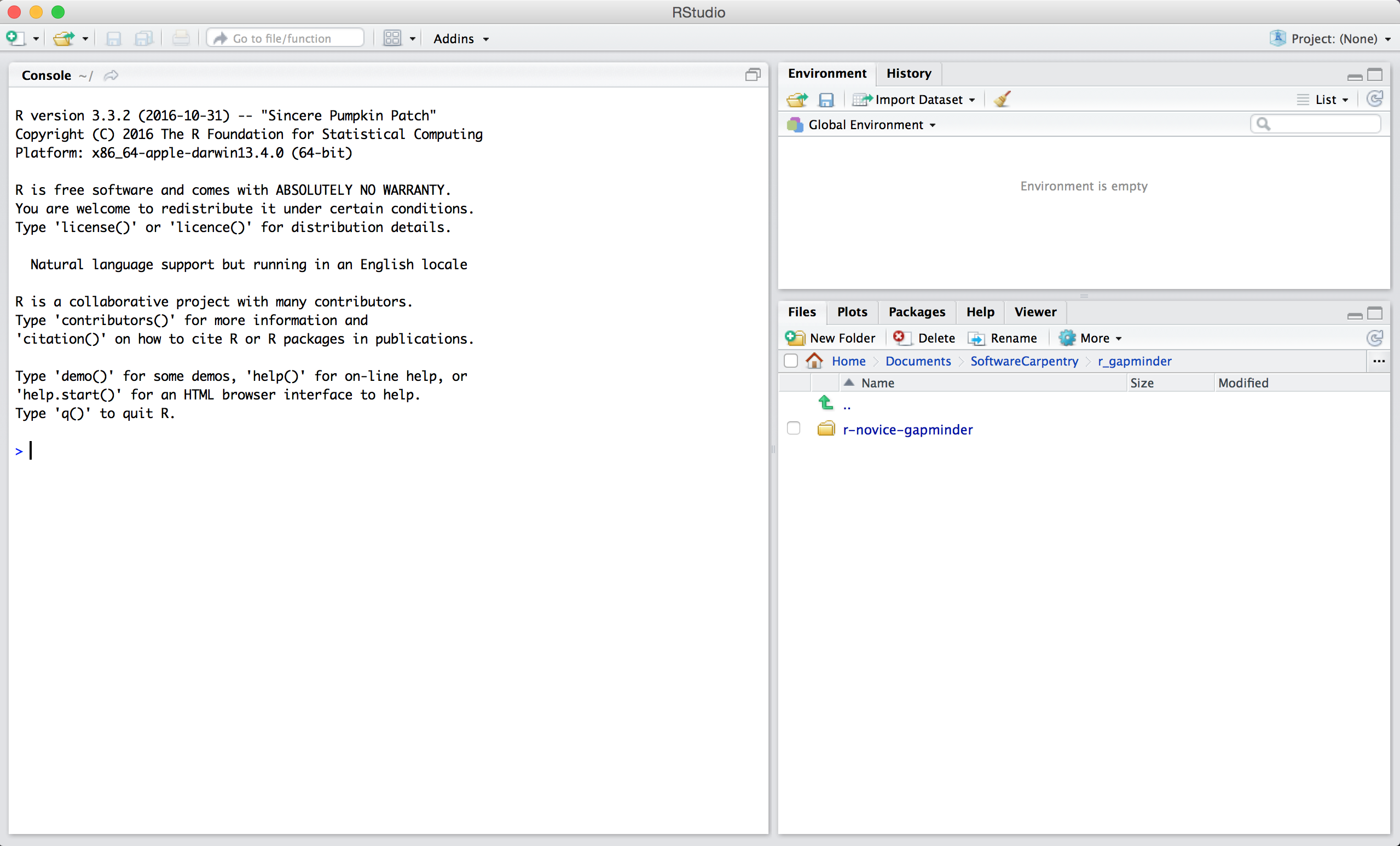
When you first open RStudio, you will be greeted by three panels:
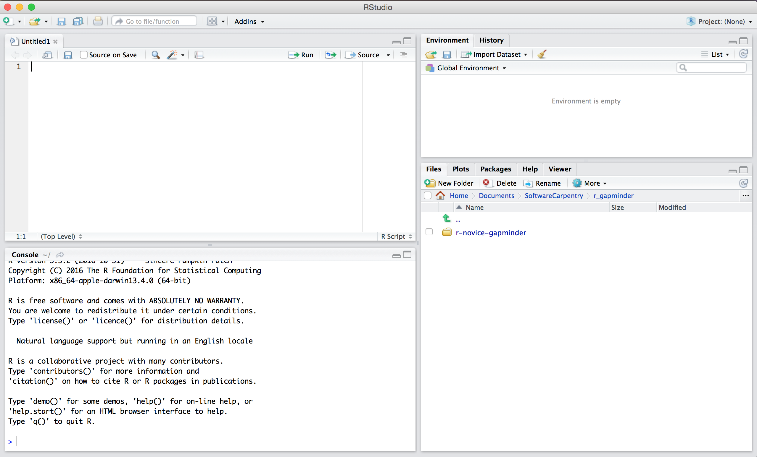
Once you open files, such as R scripts, an editor panel will also open in the top left.
There are two main ways one can work within RStudio. Both of them create an “.R” file, which is just a text file on your computer that contains a series of R commands (an R script).
source() function.Tip: Running segments of your code
RStudio offers you great flexibility in running code from within the editor window. There are buttons, menu choices, and keyboard shortcuts. To run the current line, you can
- click on the
Runbutton above the editor panel, or- select “Run Lines” from the “Code” menu, or
- hit Ctrl+Enter in Windows, Ctrl+Return in Linux, or ⌘+Return on OS X. (This shortcut can also be seen by hovering the mouse over the button). To run a block of code, select it and then
Run. If you have modified a line of code within a block of code you have just run, there is no need to reselect the section andRun, you can use the next button along,Re-run the previous region. This will run the previous code block including the modifications you have made.
Much of your time in R will be spent in the R interactive console. This is where you will run all of your code, and can be a useful environment to try out ideas before adding them to an R script file. This console in RStudio is the same as the one you would get if you typed in R in your command-line environment.
The first thing you will see in the R interactive session is a bunch of information, followed by a “>” and a blinking cursor. This where you type in commands, R tries to execute them, and then returns a result.
The simplest thing you could do with R is do arithmetic:
1 + 100And R will print out the answer, with a preceding “[1].” Don’t worry about this for now, we’ll explain that later. For now think of it as indicating output.
If you type in an incomplete command, R will wait for you to complete it:
> 1 ++Any time you hit return and the R session shows a “+” instead of a “>,” it means it’s waiting for you to complete the command. If you want to cancel a command you can simply hit “Esc” and RStudio will give you back the “>” prompt.
Tip: Cancelling commands
If you’re using R from the command line instead of from within RStudio, you need to use Ctrl+C instead of Esc to cancel the command. This applies to Mac users as well!
Cancelling a command isn’t only useful for killing incomplete commands: you can also use it to tell R to stop running code (for example if it’s taking much longer than you expect), or to get rid of the code you’re currently writing.
When using R as a calculator, the order of operations is the same as you would have learned back in school.
From highest to lowest precedence:
(, )^ or **/*+-3 + 5 * 2Use parentheses to group operations in order to force the order of evaluation if it differs from the default, or to make clear what you intend.
(3 + 5) * 2This can get unwieldy when not needed, but clarifies your intentions. Remember that others may later read your code.
(3 + (5 * (2 ^ 2))) # hard to read
3 + 5 * 2 ^ 2       # clear, if you remember the rules
3 + 5 * (2 ^ 2)     # if you forget some rules, this might help
The text after each line of code is called a “comment.” Anything that follows after the hash (or octothorpe) symbol # is ignored by R when it executes code.
Really small or large numbers get a scientific notation:
2/10000Which is shorthand for “multiplied by 10^XX.” So 2e-4 is shorthand for 2 * 10^(-4).
You can write numbers in scientific notation too:
5e3 # Note the lack of minus hereDon’t worry about trying to remember every function in R. You can look them up on Google, or if you can remember the start of the function’s name, use the tab completion in RStudio.
This is one advantage that RStudio has over R on its own, it has auto-completion abilities that allow you to more easily look up functions, their arguments, and the values that they take.
Typing a ? before the name of a command will open the help page for that command. As well as providing a detailed description of the command and how it works, scrolling to the bottom of the help page will usually show a collection of code examples which illustrate command usage. We’ll go through an example later.
We can also do comparison in R:
1 == 1 # equality (note two equals signs, read as "is equal to")1 != 2 # inequality (read as "is not equal to")1 < 2 # less than1 <= 1 # less than or equal to1 > 0 # greater than1 >= -9 # greater than or equal toTip: Comparing Numbers
A word of warning about comparing numbers: you should never use
==to compare two numbers unless they are integers (a data type which can specifically represent only whole numbers).Computers may only represent decimal numbers with a certain degree of precision, so two numbers which look the same when printed out by R, may actually have different underlying representations and therefore be different by a small margin of error (called Machine numeric tolerance).
Instead you should use the
all.equalfunction.Further reading: http://floating-point-gui.de/
We can store values in variables using the assignment operator <-, like this:
x <- 1/40Notice that assignment does not print a value. Instead, we stored it for later in something called a variable. x now contains the value 0.025:
xMore precisely, the stored value is a decimal approximation of this fraction called a floating point number.
Look for the Environment tab in one of the panes of RStudio, and you will see that x and its value have appeared. Our variable x can be used in place of a number in any calculation that expects a number:
log(x)Notice also that variables can be reassigned:
x <- 100x used to contain the value 0.025 and and now it has the value 100.
Assignment values can contain the variable being assigned to:
x <- x + 1 #notice how RStudio updates its description of x on the top right tab
y <- x * 2
The right hand side of the assignment can be any valid R expression. The right hand side is fully evaluated before the assignment occurs.
What will be the value of each variable after each statement in the following program?
mass <- 47.5
age <- 122
mass <- mass * 2.3
age <- age - 20mass <- 47.5This will give a value of r mass for the variable mass
age <- 122This will give a value of r age for the variable age
mass <- mass * 2.3This will multiply the existing value of r mass/2.3 by 2.3 to give a new value of r mass to the variable mass.
age <- age - 20This will subtract 20 from the existing value of r age + 20 to give a new value of r age to the variable age.
Run the code from the previous challenge, and write a command to compare mass to age. Is mass larger than age?
One way of answering this question in R is to use the > to set up the following:
mass > ageThis should yield a boolean value of TRUE since r mass is greater than r age.
Variable names can contain letters, numbers, underscores and periods. They cannot start with a number nor contain spaces at all. Different people use different conventions for long variable names, these include
periods.between.wordsunderscores_between_wordscamelCaseToSeparateWordsWhat you use is up to you, but be consistent.
It is also possible to use the = operator for assignment:
x = 1/40But this is much less common among R users. The most important thing is to be consistent with the operator you use. There are occasionally places where it is less confusing to use <- than =, and it is the most common symbol used in the community. So the recommendation is to use <-.
Which of the following are valid R variable names?
min_height
max.height
_age
.mass
MaxLength
min-length
2widths
celsius2kelvinThe following can be used as R variables:
min_height
max.height
MaxLength
celsius2kelvin
The following creates a hidden variable:
.massWe won’t be discussing hidden variables in this lesson. We recommend not using a period at the beginning of variable names unless you intend your variables to be hidden.
The following will not be able to be used to create a variable
_age
min-length
2widths